Tuesday, December 12, 2006

Elements of Bayesian Networks

To introduce the elements of a Bayesian network an example from animal production is used

A livestock producer has to establish as quickly as possibly, whether an animal, which has been mated, has become pregnant. If the animal is not pregnant, he has to observe the animal with extra care, to discover, when the animal returns to oestrus. If the animal is pregnant, the farmer has to adjust the feeding, to secure fulfilment of the requirements of the embryos. In addition, in dairy production the farmer will know the remaining length of the current lactation period, and can make actions e.g. in relation to milk quota. In pig production, the farmer should ensure that there is sufficient space for the sow when it is to give birth (to farrow), either in a recently cleaned pen or in an available farrowing hut.

Therefore, a pregnancy-test is usually made. The test is similar to pregnancy test of women. There are several different methods for making the test. The methods include hormone-measures in blood or urine and ultrasound-scannings.

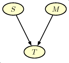
This setup can easily be modelled using Bayesian networks. In the figure below, a network is shown that represents the pregnancy-test scenario. The purpose of the network is to tell the farmer how probable it is that the sow or the cow is pregnant, when he knows the outcome of the pregnancy test.

Elements of the Bayesian network

Bayesian networks are based on so-called graphical models. The networks can model very complicated systems even though they are build using very simple building blocks. The simple structure has the advantage that the models are easy to understand. The buildings blocks are presented below. We refers to the example in the figure.

Graph Even though the network is simple, it illustrates many of the building blocks in Bayesian Networks. Thus, the ellipses in the figure are so-called nodes in the graph. A set of different states is assigned to each node. The node State has the states Not Pregnant and Pregnant. Similarly, the node Test has the states Positive and Negative assigned, corresponding to the outcome of the pregnancy test. A line connects the two nodes, a so-called edge. The arrow indicates the direction of the edge.

A node with incoming arrows from other nodes is a child of these nodes, and these are parents to the node. The node State is the only parent of the node Test,, which is a child of State. The direction of the edge indicates a causal relation. The outcome of the pregnancy test is a consequence of the state of the animal and not vice versa.

Probability In addition the the graph, you have to specify the probabilities that the nodes are in different states. With respect to nodes without parents (such as State ) the probability of each state is specified directly, e.g. based on expert knowledge or previous observations. As an example, approximately 85% of sows becomes pregnant at each mating, while the corresponding value for cows is somewhat lower (approx. 50%). In a graphical model for pregnancy testing of a sow, you would therefore specify the probability 0.15 for the state Not Pregnant and 0.85 for the state Pregnant.

For nodes with parents (such as Test ) the probability of each state is specified for the situation where the states of the parents are known. In our example, the probability of a positive test outcome should be specified for the case when the animal is pregnant, as well as the case where she is not pregnant. Typical values for these probabilities are known from other studies of pregnancy tests. The test is positive in 95% of the cases, when the sow is pregnant. If the sow is not pregnant the probability of a positive test outcome is only 30%. Of course these probabilities should be modified the reflect the precision of the specific method used for pregnancy testing.

Use of the network

When the graph and the probabilities are specified the network is ready for use. A pig producer performs a pregnancy test with a negative outcome and want to know the true state the sow. Thus he is interested in making a deduction in the opposite direction of arrow, that is from the child Test to the parent State . During the specification of the network we followed the direction of the arrow. Due to Bayes's formula it is possible to 'reverse' the calculations and make deductions in the opposite directions.

The Bayesian Network performs these calculations. Even with a negative outcome of the test, the probability of pregnancy is 29%. If the test outcome is positive this probability increases to approximately 95%.


This is based on the Danish Bedre Beslutninger med Bayesianske Net

Thomas Bayes and his Formula

Thomas Bayes (1702-1761) was a British Presbytarian minister and mathematician. He was the first to use probability calculus for inference concerning future events based on evidence. In this context he used the formula, which as now known as Bayes formula. Using a modern notation it looks like this:

$ P(D|R) =\frac{P(R|D)P(D)}{P(R | D)P(D)+P(R|\bar D)(1-P(D))}.$

In the example with the pregnancy test $P(R |D)$ and $P(R |\bar D)$ denotes the probability of the test outcome, $R$, depending on whether the sow is pregnant or not, and $P(D)$ denotes the probability that the sow is pregnant before the test result is available. On the left side of the equation, $P(D | R)$ denotes the desired probability that the sow is pregnant after the test result is known.

A bayesian network exploits a version of the formula to calculate similar probabilities in more complex frameworks.

Thomas Bayes did not publish his Essay Towards Solving a Problem in the Doctrine of Chances himself. It was published in 1763 after his dead.

See Thomas Bayes - Wikipedia, the free encyclopedia for further information.

Translated from Bayes og hans formel

Wednesday, December 06, 2006

Enhanced pregnancy testing

The value of pregnancy testing is often over-estimated, because the pregnancy test is not the only test used. After three weeks many of the non-pregnant sows will return to oestrus. Oestrus signs are a very specific indicator of non-pregnancy. If this Oestrus (heat) is detected, the pig producer knows that the sow is not pregnant and therefore, she will not make any pregnancy test of the sows. This is an example of the so-called verification bias.

Thus a more realistic example will have to include the heat detection at three weeks after mating, that is, one week before the pregnancy test

In addition, a herd level for pregnancy rate is included. We allow for the possibility of different herd levels for the pregnancy rate. A simple expansion of the net is shown in the figure below.

The graph in figure has two additional nodes.

  • $H_M$ Heat_Detection Indicates the quality of the heat detection method (corresponds to $P_M$. The node has two states (Good, Bad) with prior probabilities (0.50,0.50)
  • $H_T$ Outcome of Heat_Detection Indicates the outcome of the heat detection (corresponds to $P_T$). The node has two states ( Neg, Pos).
Finally we add one more node Herd, which gives the possibility of specifying different level for pregnancy probability in the herd. The node has 7 states (0.70, 0.75,0.80, 0.85, 0.90, 0.95, 0.975) with uniform á priori probabilities (1/7). The final extended network is shown in the figure below and can be downloaded as a Hugin netfile

GRAPPA

Again we start reading the GRAPPA code

 source("grappa.r")
Then we define $P_M$ and $H_M$
 query('PM',c(0.5,0.5))
 query('HM',c(0.5,0.5))
and the Herd node with 7 levels of pregnancy rate

 tx<-rep(1,7)/7
 pHerd<-c(0.70, 0.75,0.80, 0.85, 0.90, 0.95, 0.975)
 tab('Herd',7,tx,as.character(pHerd))
The pregnancy state node, $S$ is now a child of the Herd node. Thus the definition differ from the simple net. The conditional distribution of $P_T$ and $H_T$ is very similar to the simple net.
 # make Pregnancy state node

 tab(c('S','Herd'),c(2,7),
     as.vector(rbind(1-pHerd,pHerd)),
     c('no','yes'))

 tab(c('PT','S','PM'),, 
     c(0.85,0.15,
       0.05,0.95,
       0.65,0.35,
       0.15,0.85),c("neg","pos"))
  # Måske forkert i det oprindelige net
 tab(c('HT','S','HM'),,
     c( 0.25,0.75,
        0.5,0.5,  
        0.99,0.01,
        0.98,0.02 ),c("neg","pos"))

 vs('PM',c('Good','Bad'))
 vs('HM',c('Good','Bad'))
The initialisation step is identical

# compile, initialise and equilibrate

 compile()
 initcliqs()
 trav()
And the input of evidence just as standard. A few examples follows.


 equil()
 prop.evid('Herd','0.7')
 prop.evid('PT','neg')
 pnmarg('S')

 equil()
 prop.evid('Herd','0.7')
 prop.evid('HT','neg')
 pnmarg('S')
 prop.evid('PT','neg')
 pnmarg('S')

Verification Bias

We start with evidence on the herd level of 0.70, i.e. the same as in the simple net. If we only input a test (negative) result for the pregnancy testing we obtain the same result, that is a posterior probability of not being pregnant of 0.76. However, if we already have removed the sows with observed heat, the prior pregnancy probability before pregnancy test increases to 0.86. If the pregnancy test is negative there are still 45 % of the sows that are pregnant. Instead of the probability of not being pregnant of 0.76, it is 0.55, if we include the prior test. The magnitude of the bias depends on the pregnancy rate. By changing the evidence for the herd level this effect can be explored.

Thursday, November 23, 2006

Simple Pregnancy Testing (revisited)

A little more detailed description of the simple pregnancy testing example described here. This is a description of the network, that can be downloaded as the HUGIN netfile DRGTTEST.NET

The standard management procedure in sow production is to make a pregnancy test four weeks after mating in order to establish, whether a sow is pregnant or not. Often the farmer will know the expected pregnancy rate in the herd. The test precision will depend on the skill of the farmer. This can be modelled in a Bayesian Network (BN) as shown in the figure

The graph consists of three nodes:

  • S, Pregnancy state. Indicates the true state of the sow. The node has two states: (No, Yes). The á priori probabilities are (0.3, 0.7).
  • M, Method for pregnancy testing. Indicates the quality of the pregnancy tester. The node has two states (Good, Bad) with á priori probabilities (0.5, 0.5).
  • T, Outcome of Pregnancy Test Indicates the outcome of the pregnancy test. The node has two states (Neg, Pos) indicating a negative and a positive outcome respectively.
Method Good Bad
State no yes no yes
neg 0.85 0.15 0.65 0.15
pos 0.15 0.95 0.35 0.85

Using GRAPPA

The network is available as a Hugin netfile here, but there are several options for handling the network.

One possibility is Peter Greens GRAPPA program available for use in R, which is a free software environment for statistical computing and graphics. R can be downloaded from a CRAN mirror.

Unfortunately, GRAPPA is not available as a standard R-package, which would make it easier to install and use. But if you visit the home page you simple need to download the R source code, the Windows DLL (or the Fortran source code if you're not using Windows), and the user guide in PDF format.

Then you can proceed as follows (currently R produces some warnings, which you may ignorere).

 # load grappa source code
 source("grappa.r")

 # define the three nodes
 query('S',c(0.3,0.7))
 query('M',c(0.5,0.5))

 tab(c('T','S','M'),,
     c(0.85,0.15,
       0.05,0.95,
       0.65,0.35,
       0.15,0.85),c("neg","pos"))

 vs('S',c('no','yes'))
 vs('M',c('Good','Bad'))

# compile, initialise and equilibrate

 compile()
 initcliqs()
 trav()
Now you may use the network for inference
 # remove previous evidence 
  equil()

 # add new evidence and 
 # read the posterior probabilities
 prop.evid('T','neg')

 pnmarg('S')
 pnmarg('M')

 # If you know you are good at testing
 prop.evid('M','Good')
 pnmarg('S')

Thus, if you observe a negative test result, the probability of being non-pregnant changes from 0.3 to 0.76, and there is a slight increase in the probability that the method M is a bad method (posterior 50.8 vs the prior 50 %). If you know that the method is good, the probability of no pregnancy increases to 88 %.

Monday, November 20, 2006

Links to other BN repositories

I have just checked my del.icio.us links for other BN-repositories and have added them to the links in the left column. Currently, I have only listed three.

I will follow up with similar links to software.

Thursday, November 16, 2006

Decisions

These are examples used in the 2003 Ph.D. course Reasoning under Uncertainty in Agriculture: Bayesian Networks and Graphical Models organised by the Nordic Informatics Network in the Agricultural Sciences (Nina)

Building of expert systems.

These are examples used in the 2003 Ph.D. course Reasoning under Uncertainty in Agriculture: Bayesian Networks and Graphical Models organised by the Nordic Informatics Network in the Agricultural Sciences (Nina)

Monitoring of pregnancy rate.

This is an example used in the 2003 Ph.D. course Reasoning under Uncertainty in Agriculture: Bayesian Networks and Graphical Models organised by the Nordic Informatics Network in the Agricultural Sciences (Nina)

Monday, November 06, 2006

Simple Pregnancy Testing

  • Simple pregnancy testing (DRGTTEST.net) The standard management procedure is to make a pregnancy test four weeks after mating in order to establish whether a sow is pregnant or not. This can be modelled in a Bayesian Network (BN).
  • Enhanced pregnancy testing ( DRGTTST1.net) A more realistic example includes the heat detection at three weeks after mating, and allows for the possibility of different herd levels for the pregnancy rate.

Friday, November 03, 2006

Why Blog about Bayesian Networks in agriculture

I have gathered a lot of examples about the use of Bayesian Networks and Markov Processes during the last 15 years. They have been used for different lectures, presentations and workshops. At the moment the examples are more or less scattered on different obsolete servers and some of them on my own hard disk. My plan is to add the examples to this blog, when I have some spare time.

I realise that a wiki may be a better format for this exercise, but it was easier to set up as a blog.

My original intention was to use the name BayesianNetworks.blogspot.com but this address was already in use. As most of my examples are mainly within the agricultural domain, the addition of agriculture is not a big problem.