Prediction of productivity in Pig Herds
In Management Information Systems (MIS) for pig producers it is customary to base production control on quarterly production reports using continuous registration of productivity. The problem is how reliably such productivity records are, that is to say, how much they tell about expected future productivity.
Currently, we are constructing an expert system for herd health management decisions in slaughter pig production. In this context we need prediction models for daily gain, feed consumption and mortality.
We have a sample of data from Danish slaughter pig herds. Based on statistical analysis of these data we need to build the prediction model as a Bayesian Network. The necessary stages in this process is illustrated below. A word of caution, the data analysis is not final, and the parameter values does not necessarily reflect the Danish Production level. The examples are shown to illustrate the potential in the Bayesian Network formulation.
Statistical Model Formulation
In the data set we have the production traits in a sample of herds registered for at least 6 quarters for each herd. We want to model the variability between the herds and over time within the herd. The three variables analysed was:
- Daily gain. Corresponds to the average growth rate in gram per day in the herd. In the MIS the definition is somewhat different, but in this context we ignore this issue.
- Feed consumption rate. Corresponds to the total feed intake measured in the Danish Feed Unit for Pig per kg live weight gain. Again the MIS definition is slightly different.
- Mortality rate. Corresponds to the proportion of pigs that die before slaughter, with the similar cautionary remark about the MIS definition
The model used for the analysis is a linear normal mixed model and includes a random effect of herd, a random trend component, and additionally an auto-regressive term describing the correlation between subsequent production periods. The logit transformation was used on the mortality rate to stabilise the variance.
The full model for the analysis of daily gain is shown below, for the SAS and the R environment for statistical analysis. To investigate potential model reductions the Bayesian Information Criteria was used for model selection
SAS-specification:
 PROC MIXED METHOD=ML;
 CLASS HERD TIMEC;
 MODEL DG = TIME ;
 RANDOM INT TIME / SUBJECT=HERD TYPE=UN;
 REPEATED TIMEC / SUBJECT=HERD TYPE=AR(1) ;
lme in R.
The R-analysis is made using the lme() function in the nlme package in R.
lme(DG ~ TIME , random= ~TIME| HERD, data=HERDDATA,
 method="ML", correlation = corAR1(form=~1|HERD))
Network construction for Daily Gain
For daily gain the optimal model included only the random regression part and not the auto-regression part. Thus the resulting Bayesian Network includes only the observations (DGx), the predicted future level of Daily Gain, and the random regression parameters, Herd and Trend.
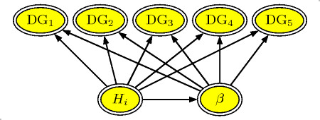
The Bayesian Network is formulated as a CG-model (Conditional Gaussian) with the structure as illustrated in the figure below.
The network contains 4 different nodes
- Herd ($H_i$) The herd's average level of daily gain
- Trend ($\beta$) The yearly change in daily gain in the herd
- DGx (DG$_i$) The (observed) daily gain in subsequent production periods. DG$_4$ is the most recent
- DGFuture. (DG$_5$ The future (predicted) daily gain in the herd.
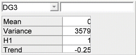
The mean daily gain DG$_i$ is the sum of the herd's level plus the herd's trend in daily gain. Thus we set the mean level in the network specification to 0, the coefficient for the herd level to 1, and the coefficient to the trend $\beta$ to $(i-4)/4$, as the time is measured in years since the current time (at step 4). The variance of the DG nodes is equal to the residual variance estimated in the statistical analysis.
The future daily gain (DG$_5$) is identical with respect to the mean level, but the residual variance is set to 0 (or 0.001 to avoid numerical problems in the analysis)
The herd level is $N(835.6,77^2)$. The estimates of the mean and the trend parameter are correlated, but we need the conditional distribution in the network. Using standard operations on the multivariate distribution we find these values ($\beta=\sigma_{AB}/sigma_{A}^{2}$ $sigma_{\res}^2=\sigma_{A}^2-\sigma_{AB}^2/sigma_{B}^2$). Thus the conditional mean the trend is $0 + 0.0126 H$ and the residual standard deviation $20$. These values are input in the specification of the trend node ($\beta$).
This completes the specification of the network. In later postings I will show the specification of the network for the other variables, and present some possibilities for the use of these networks.
Links
The specification of the network for Hugin Lite may be downloaded:
 Daily gain network


No comments:
Post a Comment