Friday, January 25, 2008

Agricultural management and Bayesian networks

Via Google Alert I got this link to a blog in Thailand. As far as I can se it is a blog used in a project concerning natural resource management. The blog includes a link to this article:

Participatory decision support for agricultural management. A case study from Sri Lanka
Agricultural Systems, Volume 76, Issue 2, May 2003
J. D. Cain, K. Jinapala, I. W. Makin, P. G. Somaratna, B. R. Ariyaratna and L. R. Perera

The reference is from 2003. The blog mentioned above included it because it has been cited a lot (13 times). If you follow the link to the citations via Google Scholar, there seem to be quite a few interesting applications within agriculture and natural management.

In fact, I found out that the Cain et al. article was one of the examples of applications in agriculture, environment and biology that we listed in connection with the Nina workshop about Reasoning under Uncertainty in Agriculture: Bayesian Networks and Graphical Models. I have referred to this workshop before, but not to the list of references. They might be of interest.

Thursday, January 10, 2008

Polar Bears and Bayesian Networks

Bayesian networks are also used within ecology and management of natural resources. Yesterday, I found a new example of this. In a recent news item in Nature, US decision on polar bear status on hold, it was described how Bayesian networks have been used to give answer to the following:

In January 2007, the wildlife service asked the US Geological Survey to address three questions: How much ice is melting, how fast is it melting, and how will this affect polar bears?

As a Dane, I have a special interest in polar bears. Denmark and Norway have had a tight connection with Greenland ever since the Erik the Red and Greenland is now a self-governing Danish province. Stories about polar bears are common in Danish litterature. To name a few: I still remember Little Nanok a childrens book by Elmar Drastrup, about the troublesome life of a polar bear cub, and Jørn Riel has written some excellent collections of 'tall' stories from Greenland. Some of them seems to have been translated at least into French and German.

In addition, a standard urban myth(?) describes how foreigners believe that polar bears roam the streets of Copenhagen. The story is actually used as the opening lines in Anna's Book by Ruth Rendell: "When I went out this morning a woman asked me if there were polar bears in the streets of Copenhagen...". The Flickr image shown here of the polar bear is indeed from Copenhagen, but from the zoo.

But this has very little to do with Bayesian Networks

So I will return my focus with another quote from the Nature article:

Answering those seemingly simple questions [quoted above] was a challenge, not only because the future climate is difficult to predict, but also because data on the bears is so meagre. Little is known about the bears that live in the most remote regions, such as the Arctic basin at the very top of the world. Among the 19 subpopulations found throughout the Arctic, there are three whose numbers have never been counted and are unknown.

"The goal was to try and extract the maximum amount of information from the data that we do have," says Steven Amstrup, who leads the polar bear research group at the US Geological Survey in Anchorage, Alaska.

Amstrup and colleagues have assessed the effects of individual stressors, such as hunting and ice loss, and used a ‘Bayesian network model’ to estimate the likelihood of different outcomes to the stressors. They found that declining sea ice overrode all other factors, and that several populations of polar bears, including those found along the southern Beaufort Sea, north of Alaska, were likely to vanish by the end of this century.

A very detailed description of the network can be found in the report Forecasting the Range-wide Status of Polar Bears at Selected Times in the 21st century.(pdf-file) by Steven C. Amstrup, Bruce G. Marcot, and David C. Douglas.

The Bayesian Network models how different stressors influence the polar bear population and the network was based on expert-input from S. Amstrup concerning the model structure and the relevant tables of conditional probabilities. The nodes of the network were divided into three kinds. 1) the input nodes representing anthropogenic stressors and environmental variables. 2) Summary nodes combining the efects of the different stressor, and 3) the output nodes, i.e., nodes describng the effect on population size and structure. The figure shown below is a copy of Figure 4 in the report. The figure illustrates the relation between the nodes in network

My search for further information concerning the research led me to this page concerning Bayesian Network Models in Ecology by one of the authors of the report, Bruce G. Marcot. He was the knowledge engineer in the study. The home page includes several interesting links

Amstrup and other -trups

I started on the irrelevant mood, and this final section is to maintain the symmetry. I am almost certain that Steven Amstrup is a descendant of Danish emmigrants. Amstrup is the name of at least 3 Danish villages, and follows a standard construction of Danish village names, which was very common in Denmark just in the period following the viking age. The construction is: name plus -strup/torp/-rup. The original ending -torp probably refers to a new settlement for people that have left an older village. Within a radius of approximately 20 km around my hometown, we have Knabstrup, Algestrup, Gundestrup, Jyderup, Allerup, Tåstrup, Ordrup, Søstrup, Sasserup, Hellestrup, Butterup, Borup, ...., Regstrup, but no Amstrup, that name seem to be used primarily in Jutland. And the nearest is just 20 km away from our Research Centre, close to Ulstrup

Monday, January 08, 2007

Prediction of productivity in Pig Herds

In Management Information Systems (MIS) for pig producers it is customary to base production control on quarterly production reports using continuous registration of productivity. The problem is how reliably such productivity records are, that is to say, how much they tell about expected future productivity.

Currently, we are constructing an expert system for herd health management decisions in slaughter pig production. In this context we need prediction models for daily gain, feed consumption and mortality.

We have a sample of data from Danish slaughter pig herds. Based on statistical analysis of these data we need to build the prediction model as a Bayesian Network. The necessary stages in this process is illustrated below. A word of caution, the data analysis is not final, and the parameter values does not necessarily reflect the Danish Production level. The examples are shown to illustrate the potential in the Bayesian Network formulation.

Statistical Model Formulation

In the data set we have the production traits in a sample of herds registered for at least 6 quarters for each herd. We want to model the variability between the herds and over time within the herd. The three variables analysed was:

  • Daily gain. Corresponds to the average growth rate in gram per day in the herd. In the MIS  the  definition is somewhat different, but in this context we ignore this issue.
  • Feed consumption rate. Corresponds to the total feed intake measured in the Danish Feed Unit for Pig per kg live weight gain. Again the MIS definition is slightly different.
  • Mortality rate. Corresponds to the proportion of pigs that die before slaughter, with the similar cautionary remark about the MIS definition

The model used for the analysis is a linear normal mixed model and includes a random effect of herd, a random trend component, and additionally an auto-regressive term describing the correlation between subsequent production periods. The logit transformation was used on the mortality rate to stabilise the variance.

The full model for the analysis of daily gain is shown below, for the SAS and the R environment for statistical analysis. To investigate potential model reductions the Bayesian Information Criteria was used for model selection

SAS-specification:

 
 PROC MIXED METHOD=ML; 
 CLASS HERD TIMEC; 
 MODEL DG = TIME ;
 RANDOM INT TIME / SUBJECT=HERD TYPE=UN; 
 REPEATED TIMEC / SUBJECT=HERD TYPE=AR(1) ; 

lme in R.

The R-analysis is made using the lme() function in the nlme package in R.

lme(DG ~ TIME , random= ~TIME| HERD, data=HERDDATA,
method="ML", correlation = corAR1(form=~1|HERD))
 

Network construction for Daily Gain

For daily gain the optimal model included only the random regression part and not the auto-regression part. Thus the resulting Bayesian Network includes only the observations (DGx), the predicted future level of Daily Gain, and the random regression parameters, Herd and Trend.

The Bayesian Network is formulated as a CG-model (Conditional Gaussian) with the structure as illustrated in the figure below.

The network contains 4 different nodes

  • Herd ($H_i$) The herd's average level of daily gain
  • Trend ($\beta$) The yearly change in daily gain in the herd
  • DGx (DG$_i$) The (observed) daily gain in subsequent production periods. DG$_4$ is the most recent
  • DGFuture. (DG$_5$ The future (predicted) daily gain in the herd.

DailyGain450 Daily gain network

The mean daily gain DG$_i$ is the sum of the herd's level plus the herd's trend in daily gain. Thus we set the mean level in the network specification to 0, the coefficient for the herd level to 1, and the coefficient to the trend $\beta$ to $(i-4)/4$, as the time is measured in years since the current time (at step 4). The variance of the DG nodes is equal to the residual variance estimated in the statistical analysis.

dgtablefinal

The future daily gain (DG$_5$) is identical with respect to the mean level, but the residual variance is set to 0 (or 0.001 to avoid numerical problems in the analysis)

The herd level is $N(835.6,77^2)$. The estimates of the mean and the trend parameter are correlated, but we need the conditional distribution in the network. Using standard operations on the multivariate distribution we find these values ($\beta=\sigma_{AB}/sigma_{A}^{2}$ $sigma_{\res}^2=\sigma_{A}^2-\sigma_{AB}^2/sigma_{B}^2$). Thus the conditional mean the trend is $0 + 0.0126 H$ and the residual standard deviation $20$. These values are input in the specification of the trend node ($\beta$).

This completes the specification of the network. In later postings I will show the specification of the network for the other variables, and present some possibilities for the use of these networks.

Links

The specification of the network for Hugin Lite may be downloaded:

Tuesday, December 12, 2006

Elements of Bayesian Networks

To introduce the elements of a Bayesian network an example from animal production is used

A livestock producer has to establish as quickly as possibly, whether an animal, which has been mated, has become pregnant. If the animal is not pregnant, he has to observe the animal with extra care, to discover, when the animal returns to oestrus. If the animal is pregnant, the farmer has to adjust the feeding, to secure fulfilment of the requirements of the embryos. In addition, in dairy production the farmer will know the remaining length of the current lactation period, and can make actions e.g. in relation to milk quota. In pig production, the farmer should ensure that there is sufficient space for the sow when it is to give birth (to farrow), either in a recently cleaned pen or in an available farrowing hut.

Therefore, a pregnancy-test is usually made. The test is similar to pregnancy test of women. There are several different methods for making the test. The methods include hormone-measures in blood or urine and ultrasound-scannings.

This setup can easily be modelled using Bayesian networks. In the figure below, a network is shown that represents the pregnancy-test scenario. The purpose of the network is to tell the farmer how probable it is that the sow or the cow is pregnant, when he knows the outcome of the pregnancy test.

Elements of the Bayesian network

Bayesian networks are based on so-called graphical models. The networks can model very complicated systems even though they are build using very simple building blocks. The simple structure has the advantage that the models are easy to understand. The buildings blocks are presented below. We refers to the example in the figure.

Graph Even though the network is simple, it illustrates many of the building blocks in Bayesian Networks. Thus, the ellipses in the figure are so-called nodes in the graph. A set of different states is assigned to each node. The node State has the states Not Pregnant and Pregnant. Similarly, the node Test has the states Positive and Negative assigned, corresponding to the outcome of the pregnancy test. A line connects the two nodes, a so-called edge. The arrow indicates the direction of the edge.

A node with incoming arrows from other nodes is a child of these nodes, and these are parents to the node. The node State is the only parent of the node Test,, which is a child of State. The direction of the edge indicates a causal relation. The outcome of the pregnancy test is a consequence of the state of the animal and not vice versa.

Probability In addition the the graph, you have to specify the probabilities that the nodes are in different states. With respect to nodes without parents (such as State ) the probability of each state is specified directly, e.g. based on expert knowledge or previous observations. As an example, approximately 85% of sows becomes pregnant at each mating, while the corresponding value for cows is somewhat lower (approx. 50%). In a graphical model for pregnancy testing of a sow, you would therefore specify the probability 0.15 for the state Not Pregnant and 0.85 for the state Pregnant.

For nodes with parents (such as Test ) the probability of each state is specified for the situation where the states of the parents are known. In our example, the probability of a positive test outcome should be specified for the case when the animal is pregnant, as well as the case where she is not pregnant. Typical values for these probabilities are known from other studies of pregnancy tests. The test is positive in 95% of the cases, when the sow is pregnant. If the sow is not pregnant the probability of a positive test outcome is only 30%. Of course these probabilities should be modified the reflect the precision of the specific method used for pregnancy testing.

Use of the network

When the graph and the probabilities are specified the network is ready for use. A pig producer performs a pregnancy test with a negative outcome and want to know the true state the sow. Thus he is interested in making a deduction in the opposite direction of arrow, that is from the child Test to the parent State . During the specification of the network we followed the direction of the arrow. Due to Bayes's formula it is possible to 'reverse' the calculations and make deductions in the opposite directions.

The Bayesian Network performs these calculations. Even with a negative outcome of the test, the probability of pregnancy is 29%. If the test outcome is positive this probability increases to approximately 95%.


This is based on the Danish Bedre Beslutninger med Bayesianske Net

Thomas Bayes and his Formula

Thomas Bayes (1702-1761) was a British Presbytarian minister and mathematician. He was the first to use probability calculus for inference concerning future events based on evidence. In this context he used the formula, which as now known as Bayes formula. Using a modern notation it looks like this:

$ P(D|R) =\frac{P(R|D)P(D)}{P(R | D)P(D)+P(R|\bar D)(1-P(D))}.$

In the example with the pregnancy test $P(R |D)$ and $P(R |\bar D)$ denotes the probability of the test outcome, $R$, depending on whether the sow is pregnant or not, and $P(D)$ denotes the probability that the sow is pregnant before the test result is available. On the left side of the equation, $P(D | R)$ denotes the desired probability that the sow is pregnant after the test result is known.

A bayesian network exploits a version of the formula to calculate similar probabilities in more complex frameworks.

Thomas Bayes did not publish his Essay Towards Solving a Problem in the Doctrine of Chances himself. It was published in 1763 after his dead.

See Thomas Bayes - Wikipedia, the free encyclopedia for further information.

Translated from Bayes og hans formel

Wednesday, December 06, 2006

Enhanced pregnancy testing

The value of pregnancy testing is often over-estimated, because the pregnancy test is not the only test used. After three weeks many of the non-pregnant sows will return to oestrus. Oestrus signs are a very specific indicator of non-pregnancy. If this Oestrus (heat) is detected, the pig producer knows that the sow is not pregnant and therefore, she will not make any pregnancy test of the sows. This is an example of the so-called verification bias.

Thus a more realistic example will have to include the heat detection at three weeks after mating, that is, one week before the pregnancy test

In addition, a herd level for pregnancy rate is included. We allow for the possibility of different herd levels for the pregnancy rate. A simple expansion of the net is shown in the figure below.

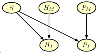
The graph in figure has two additional nodes.

  • $H_M$ Heat_Detection Indicates the quality of the heat detection method (corresponds to $P_M$. The node has two states (Good, Bad) with prior probabilities (0.50,0.50)
  • $H_T$ Outcome of Heat_Detection Indicates the outcome of the heat detection (corresponds to $P_T$). The node has two states ( Neg, Pos).
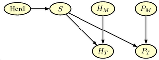
Finally we add one more node Herd, which gives the possibility of specifying different level for pregnancy probability in the herd. The node has 7 states (0.70, 0.75,0.80, 0.85, 0.90, 0.95, 0.975) with uniform á priori probabilities (1/7). The final extended network is shown in the figure below and can be downloaded as a Hugin netfile

GRAPPA

Again we start reading the GRAPPA code

 source("grappa.r")
Then we define $P_M$ and $H_M$
 query('PM',c(0.5,0.5))
 query('HM',c(0.5,0.5))
and the Herd node with 7 levels of pregnancy rate

 tx<-rep(1,7)/7
 pHerd<-c(0.70, 0.75,0.80, 0.85, 0.90, 0.95, 0.975)
 tab('Herd',7,tx,as.character(pHerd))
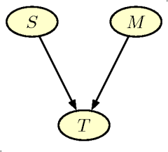
The pregnancy state node, $S$ is now a child of the Herd node. Thus the definition differ from the simple net. The conditional distribution of $P_T$ and $H_T$ is very similar to the simple net.
 # make Pregnancy state node

 tab(c('S','Herd'),c(2,7),
     as.vector(rbind(1-pHerd,pHerd)),
     c('no','yes'))

 tab(c('PT','S','PM'),, 
     c(0.85,0.15,
       0.05,0.95,
       0.65,0.35,
       0.15,0.85),c("neg","pos"))
  # Måske forkert i det oprindelige net
 tab(c('HT','S','HM'),,
     c( 0.25,0.75,
        0.5,0.5,  
        0.99,0.01,
        0.98,0.02 ),c("neg","pos"))

 vs('PM',c('Good','Bad'))
 vs('HM',c('Good','Bad'))
The initialisation step is identical

# compile, initialise and equilibrate

 compile()
 initcliqs()
 trav()
And the input of evidence just as standard. A few examples follows.


 equil()
 prop.evid('Herd','0.7')
 prop.evid('PT','neg')
 pnmarg('S')

 equil()
 prop.evid('Herd','0.7')
 prop.evid('HT','neg')
 pnmarg('S')
 prop.evid('PT','neg')
 pnmarg('S')

Verification Bias

We start with evidence on the herd level of 0.70, i.e. the same as in the simple net. If we only input a test (negative) result for the pregnancy testing we obtain the same result, that is a posterior probability of not being pregnant of 0.76. However, if we already have removed the sows with observed heat, the prior pregnancy probability before pregnancy test increases to 0.86. If the pregnancy test is negative there are still 45 % of the sows that are pregnant. Instead of the probability of not being pregnant of 0.76, it is 0.55, if we include the prior test. The magnitude of the bias depends on the pregnancy rate. By changing the evidence for the herd level this effect can be explored.
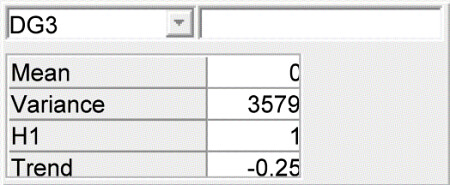
Thursday, November 23, 2006

Simple Pregnancy Testing (revisited)

A little more detailed description of the simple pregnancy testing example described here. This is a description of the network, that can be downloaded as the HUGIN netfile DRGTTEST.NET

The standard management procedure in sow production is to make a pregnancy test four weeks after mating in order to establish, whether a sow is pregnant or not. Often the farmer will know the expected pregnancy rate in the herd. The test precision will depend on the skill of the farmer. This can be modelled in a Bayesian Network (BN) as shown in the figure

The graph consists of three nodes:

  • S, Pregnancy state. Indicates the true state of the sow. The node has two states: (No, Yes). The á priori probabilities are (0.3, 0.7).
  • M, Method for pregnancy testing. Indicates the quality of the pregnancy tester. The node has two states (Good, Bad) with á priori probabilities (0.5, 0.5).
  • T, Outcome of Pregnancy Test Indicates the outcome of the pregnancy test. The node has two states (Neg, Pos) indicating a negative and a positive outcome respectively.
Method Good Bad
State no yes no yes
neg 0.85 0.15 0.65 0.15
pos 0.15 0.95 0.35 0.85

Using GRAPPA

The network is available as a Hugin netfile here, but there are several options for handling the network.

One possibility is Peter Greens GRAPPA program available for use in R, which is a free software environment for statistical computing and graphics. R can be downloaded from a CRAN mirror.

Unfortunately, GRAPPA is not available as a standard R-package, which would make it easier to install and use. But if you visit the home page you simple need to download the R source code, the Windows DLL (or the Fortran source code if you're not using Windows), and the user guide in PDF format.

Then you can proceed as follows (currently R produces some warnings, which you may ignorere).

 # load grappa source code
 source("grappa.r")

 # define the three nodes
 query('S',c(0.3,0.7))
 query('M',c(0.5,0.5))

 tab(c('T','S','M'),,
     c(0.85,0.15,
       0.05,0.95,
       0.65,0.35,
       0.15,0.85),c("neg","pos"))

 vs('S',c('no','yes'))
 vs('M',c('Good','Bad'))

# compile, initialise and equilibrate

 compile()
 initcliqs()
 trav()
Now you may use the network for inference
 # remove previous evidence 
  equil()

 # add new evidence and 
 # read the posterior probabilities
 prop.evid('T','neg')

 pnmarg('S')
 pnmarg('M')

 # If you know you are good at testing
 prop.evid('M','Good')
 pnmarg('S')

Thus, if you observe a negative test result, the probability of being non-pregnant changes from 0.3 to 0.76, and there is a slight increase in the probability that the method M is a bad method (posterior 50.8 vs the prior 50 %). If you know that the method is good, the probability of no pregnancy increases to 88 %.