Simple Pregnancy Testing (revisited)

A little more detailed description of the simple pregnancy testing example described here. This is a description of the network, that can be downloaded as the HUGIN netfile DRGTTEST.NET

The standard management procedure in sow production is to make a pregnancy test four weeks after mating in order to establish, whether a sow is pregnant or not. Often the farmer will know the expected pregnancy rate in the herd. The test precision will depend on the skill of the farmer. This can be modelled in a Bayesian Network (BN) as shown in the figure

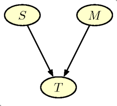
The graph consists of three nodes:

• S, Pregnancy state. Indicates the true state of the sow. The node has two states: (No, Yes). The á priori probabilities are (0.3, 0.7).
• M, Method for pregnancy testing. Indicates the quality of the pregnancy tester. The node has two states (Good, Bad) with á priori probabilities (0.5, 0.5).
• T, Outcome of Pregnancy Test Indicates the outcome of the pregnancy test. The node has two states (Neg, Pos) indicating a negative and a positive outcome respectively.

Method	Good		Bad
State	no	yes	no	yes
neg	0.85	0.15	0.65	0.15
pos	0.15	0.95	0.35	0.85

Using GRAPPA

The network is available as a Hugin netfile here, but there are several options for handling the network.

One possibility is Peter Greens GRAPPA program available for use in R, which is a free software environment for statistical computing and graphics. R can be downloaded from a CRAN mirror.

Unfortunately, GRAPPA is not available as a standard R-package, which would make it easier to install and use. But if you visit the home page you simple need to download the R source code, the Windows DLL (or the Fortran source code if you're not using Windows), and the user guide in PDF format.

Then you can proceed as follows (currently R produces some warnings, which you may ignorere).

 # load grappa source code
 source("grappa.r")

 # define the three nodes
 query('S',c(0.3,0.7))
 query('M',c(0.5,0.5))

 tab(c('T','S','M'),,
     c(0.85,0.15,
       0.05,0.95,
       0.65,0.35,
       0.15,0.85),c("neg","pos"))

 vs('S',c('no','yes'))
 vs('M',c('Good','Bad'))

# compile, initialise and equilibrate

 compile()
 initcliqs()
 trav()

Now you may use the network for inference

 # remove previous evidence 
  equil()

 # add new evidence and 
 # read the posterior probabilities
 prop.evid('T','neg')

 pnmarg('S')
 pnmarg('M')

 # If you know you are good at testing
 prop.evid('M','Good')
 pnmarg('S')

Thus, if you observe a negative test result, the probability of being non-pregnant changes from 0.3 to 0.76, and there is a slight increase in the probability that the method M is a bad method (posterior 50.8 vs the prior 50 %). If you know that the method is good, the probability of no pregnancy increases to 88 %.